In my last post I explained mathematically how Q-Learning allows us to solve any Markov Decision Process without knowing the transition function. In my final post, I'm going to finally show how Reinforcement Learning (specifically Q-Learning) works against our Very Simple Maze™. And then I'll show how the very same algorithm can also make stock market long/short decisions by simply turning the stock market into a Markov Decision Process.
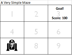
So let's start by putting a robot into our Very Simple Maze™:
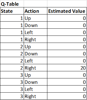
And also we're starting with a Q-function that starts out with all zeros:
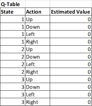
Now this robot starts to follow the 'estimated policy' which at this point just says that all actions within all states have a value of zero. In essence, it's just picking random moves. The robot wanders around and, by chance, ends up in state 2 at some point:
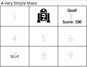
Now the robot happens to pick 'right' as it's action and by chance finds the goal and scores 100 points:
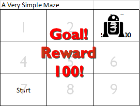
So we're going to update our Q-table (Q-function) now based on that reward. What we'll do is take 80% of the old value of the Q-table and move it part way to the reward received plus the best utility of the next state (which in this case is the goal.)
Q[s, a] = (0.8 * Q[s, a]) + (0.2 * (reward + 0.9 * Max Q[s_prime, a_prime]))
Q[2, R] = (0.8 * Q[s, a]) + (0.2 * (reward + 0.9 * Max Q[s_prime, a_prime]))
Q[2, R] = (0.8 * 0) + (0.2 * (100 + 0.9 * 0))
Q[2, R] = 20
So this updates the Q-table to be:
So then the robot starts back at start and runs through the maze again and this time randomly ends up at State 1 and randomly picks to move to State 2. When this happens, it now sees that the best utility of an action available in state 2 is now 20 instead of zero. And updates state 1 like this:
Q[s, a] = (0.8 * Q[s, a]) + (0.2 * (reward + 0.9 * Max Q[s_prime, a_prime]))
Q[1, U] = (0.8 * Q[s, a]) + (0.2 * (reward + 0.9 * Max Q[s_prime, a_prime]))
Q[1, U] = (0.8 * 0) + (0.2 * (0 + 0.9 * 20))
Q[1, R] = 3.6
So now our Q-table looks like this:
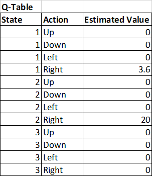
Notice that now, should our robot ever find itself back at State 1, it now will know to go to State 2, and from there know to go to State 3 and will find the goal.
So what happens when the robot moves into the goal again? Well, we get the following update to the Q-Table:
Q[s, a] = (0.8 * Q[s, a]) + (0.2 * (reward + 0.9 * Max Q[s_prime, a_prime]))
Q[2, R] = (0.8 * Q[s, a]) + (0.2 * (reward + 0.9 * Max Q[s_prime, a_prime]))
Q[2, R] = (0.8 * 20) + (0.2 * (100 + 0.9 * 0))
Q[2, R] = 36
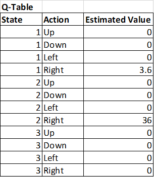
Can you see where this is going? The value of the reward is slowly flowing backwards out through the maze and will eventually find the start state! The Q-table is slowly converging towards a set of values where the robot is able to find the best path through the maze. The whole process just magically takes place and is guaranteed to converge to the correct optimal policy.
The Explore / Exploit Trade-off
Now you might notice one problem: What if the robot accidentally finds a less than optimal path through the maze first? That's okay. What we do is what's known as the "explore/exploit trade off." Basically, make a random move part of the time and follow your current best policy part of the time.
Better yet, start out taking a random move 99% of the time and following the best policy 1% of the time and then slowly shift that over time towards making fewer random moves. The end result is the robot will explore the maze enough that something close to the optimal policy will be found.
Convergence
So perhaps, many iterations later, our Q-table (Q-function) now looks like this:
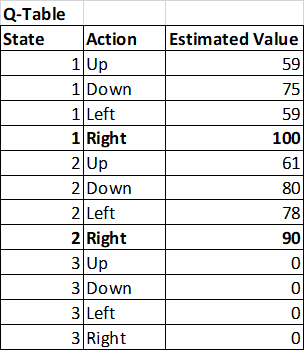
Notice how now it's very clear which action is the best one from a given state and that it's converging towards the same values as Dynamic Programming did.
This is, in essence, how Q-Learning works.
Q-Learning and the Stock Market
So I promised I'd show how to use the same Q-Learning Algorithm to do stock market predictions. So here is a quick overview of how that would work.
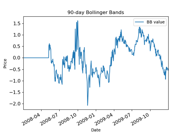
The first thing you need to do is to imagine the stock market as a set of states. One way to do that might be to track various technical signals in discrete states. So, for example, let's say you want to take a 90-day Bollinger Band signal that looks like this:
And turn it into a discrete version like this:
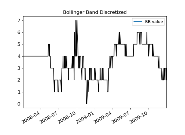
Now it's probably not a wise idea to try to model a stock using only a Bollinger Band as a signal with only 8 states, but imagine adding several other technical signals and then creating states that track across all of them simultaneously. When I did this in real life, I made 5 signals for a stock that each had 10 states. That works out to be 10^5 or 100,000 states. Still manageable.
Now here is the beauty of it: our Q-Learner we defined above just doesn't care what type of problem it's solving. It will just as gladly solve the problem of finding it's way through a maze as finding the best time to buy and sell stock. So by letting the Q-Learner run through the history of a stock and learn to maximize it's reward in terms of value of it's portfolio it will eventually come up with a policy for when to buy and sell stocks. Mine looked like this:
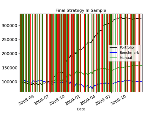
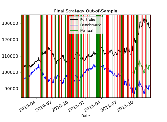
The green vertical lines were buy decisions and the red vertical lines were short decisions. The end result was that it made a lot of hypothetical money - at least using the training data. Even when I ran it against non-training data, it still did better than the benchmark:
I hope this demonstration gives you a good intuition for how and why Reinforcement Learning works. I think the truly exciting things about Reinforcement learning are:
It doesn't need labeled data like supervised learning
It continually learns even after training is finished
It is a single algorithm that can solve any type of problem once the problem has been defined as a Markov Decision Process