In my last post I situated Reinforcement Learning in the family of Artificial Intelligence vs Machine Learning group of algorithms and then described how, at least in principle, every problem can be framed in terms of the Markov Decision Process (MDP) and even described an “all purpose” (not really) algorithm for solving all MDPs – if you have happen to know the transition function (and reward function) of the problem you’re trying to solve.
But what if you don’t know the transition function?
This post is going to be a bit math heavy. But don’t worry, it’s not nearly as difficult as the fancy equations first make it seem. What I’m going to demonstrate is that using the Bellman equations (named after Richard Bellman who I mentioned in the previous post as the inventor of Dynamic Programming) and a little mathematical ingenuity, it’s actually possible to solve (or rather approximately solve) a Markov Decision Process without knowing the Transition Function or Reward Function!
The Value, Reward, and Transition Functions
So let’s start with a quick review:
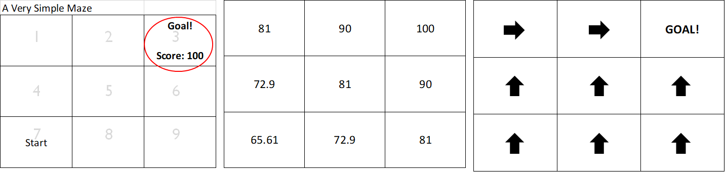
Reward Function: A function that tells us the reward of a given state. For our Very Simple Maze™ it was essentially “if you’re in state 3, return 100 otherwise return 0”
Transition Function: The transition function was just a table that told us “if you’re in state 2 and you move right you’ll now be in state 3.”
Value Function: The value function is a function we built using Dynamic Programming that calculated a Utility for each state such that we know how close we were to the goal.
Optimal Policy: A policy for each state that gets you to the highest reward as quickly as possible.
So I want to introduce one more simple idea on top of those. It’s called the Q-Function and it looks something like this:
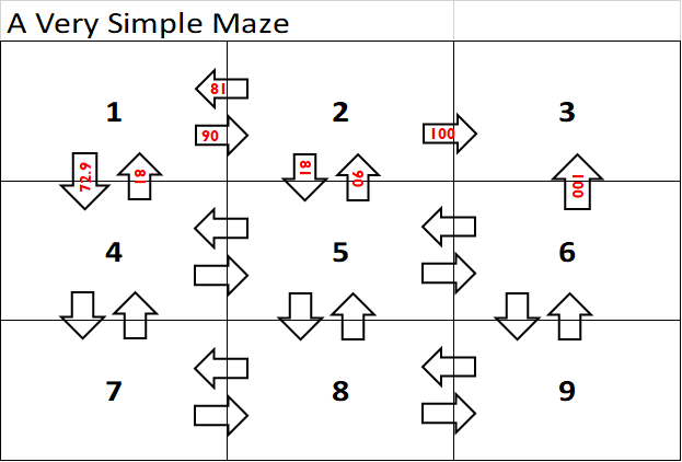
The basic idea is that it’s a lot like our value function, where we list the utility of each state based on the best possible action from that state. Here, instead, we’re listing the utility per actionfor that state. So, for example, State 2 has a utility of 100 if you move right because it gets you a reward of 100, but moving down in State 2 is a utility of only 81 because it moves you further away from the goal. So the Q-function is basically identical to the value function except it is a function of state andaction rather than just state.
It’s not hard to see that the Q-Function can be easily turned into the value function (just take the highest utility move for that state) but that the reverse isn’t true. Because of this, the Q-Function allows us to do a bit more with it and will play a critical role in how we solve MDPs without knowing the transition function.
The Beautiful Mathematical Proof
Okay, so let’s move on and I’ll now present the rest of the proof that it’s possible to solve MDPs without the transition function known. Consider this equation here:
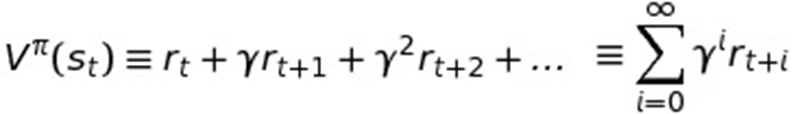
V represents the "Value function" and the PI (π) symbol represents a policy, though not (yet) necessarily the optimal policy. The γ is the Greek letter gamma and it is used to represent any time we are discounting the future.
So this fancy equation really just says that the value function for some policy, which is a function of State at time t (St), is really just the sum of rewards of that state plus the discounted (γ) rewards for every state that the policy (π) will enter into after that state. (Note how we raise the exponent on the discount γ for each additional move into the future to make each move into the future further discounted.) That final value is the value or utility of the state S at time t.
So the value function returns the utility for a state given a certain policy (π) by calculating what in economics would be called the “net present value” of the future expected rewards given the policy. It’s not hard to see that the end result would be what we’ve been calling the value function (i.e. the grid with the utilities listed for each state.) So this equation just formally explains how to calculate the value of a policy.
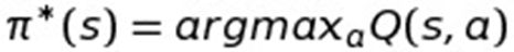
Now this would be how we calculate the value or utility of any given policy, even a bad one. But what we're really interested in is the best policy (or rather the optimal policy) that gets us the best value for a given state. So let's define what we mean by 'optimal policy':

Again, we're using the pi (π) symbol to represent a policy, but we're now placing a star above it to indicate we're now talking about the optimal policy.
So this function says that the optimal policy (π*) is the policy that returns the optimal value (or max value) possible for state "s" out of all possible States. Again, despite the weird mathematical notation, this is actually pretty intuitive so far. This basically boils down to saying that the optimal policy is the policy with the best utility from the state you are currently in. It’s thus identical to what we’ve been calling the optimal policy where you always know the best move for a given state.

This next function is actually identical to the one before (though it may not be immediately obvious that is the case) except now we're defining the optimal policy in terms of State "s". This will be handy for us later.
So this function says that the optimal policy for state "s" is the action "a" that returns the highest reward (i.e. argmax) for state "s" and action "a" plus the discounted (γ) utility of the new state you end up in. (Remember δ is the transition function, so this is just a fancy way of saying “the next state” after State "s" if you took Action "a").
In plain English this is far more intuitively obvious. It just says that the optimal policy for state "s" is the best action that gives the highest reward plus the discounted future rewards. Of course the optimal policy is that you take the best action for each state! So this one is straightforwardly obvious as well.

Okay, now we’re defining the Q-Function, which is just the reward for the current State "s" given a specific action "a", i.e. r(s,a), plus the discounted (γ) optimal value for the next state (i.e. the transition (δ) function again, which puts you into the next state when you’re in state "s" and take action "a".)
So this is basically identical to the optimal policy function right above it except now the function is based on the state and action pair rather than just state. It will become useful later that we can define the Q-function this way.
The Clever Part
Now here is where smarter people than I started getting clever:
Okay, we’re now defining the optimal policy function in terms of the Q-Function! It basically just says that the optimal policy function is equivalent to the Q function where you happen to always take the action that will return the highest value for a given state.
This is basically equivalent to how I already pointed out that the value function can be computed from the Q-Function. We already knew we could compute the optimal policy from the optimal value function, so this is really just a fancy way of saying that given you can compute the optimal policy from the optimal value function and given that you can compute the optimal value function with the Q-function, it’s therefore possible to define the optimal policy in terms of the Q-function. Not much else going on here.
So now think about this. If the optimal policy can be determined from the Q-Function, can you define the optimal value function from it? Of course you can! You just take the best (or Max) utility for a given state:
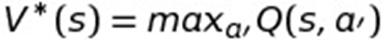
Here, the way I wrote it, "a’" means the next action you’ll take. In other words, you’re already looking at a value for the action "a" that got you to the current state, so "a’" just is a way to make it clear that we’re now talking about the next action. It’s not really saying anything else more fancy here.The bottom line is that it's entirely possible to define the optimal value function in terms of the Q-function.
So we now have the optimal value function defined in terms of the Q function. So what does that give us? As it turns out A LOT!!
Because now all we need to do is take the original Q-Function above, which was by definition defined in terms of the optimal value function, and you can replace the original value function with the above function where we're defining the Value function in terms of the Q-function.
In other words, it’s mathematically possible to define the Q-Function in terms of itself using recursion! And here is what you get:

“But wait!” I hear you cry. You haven’t accomplished anything! I mean I can still see that little transition function (δ) in the definition! So you’ve bought nothing so far! You’ve totally failed, Bruce!
But have I?
So as it turns out, now that we've defined the Q-function in terms of itself, we can do a little trick that drops the transition function out.
Estimating the Transition Function
Specifically, what we're going to do, is we'll start with an estimate of the Q-function and then slowly improve it each iteration. It's possible to show (that I won't in this post) that this is guaranteed over time (after infinity iterations) to converge to the real values of the Q-function.
Wait, infinity iterations? Yeah, but you will end up with an approximate result long before infinity.
But here is the algorithm in question:
Q-Learning Algorithm:
Select an action a and execute it (part of the time select at random, part of the time, select what currently is the best known action from the Q-function tables)
Receive immediate reward r
Observe the new state s' (s' become new s)
Update the table entry as follows:
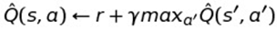
This equation really just says that you have a table containing the Q-function and you update that table with each move by taking the reward for the last State s / Action a pair and add it to the max valued action (a') of the new state you wind up in (i.e. the utility of that state.) Notice how it's very similar to the recursively defined Q-function.
So in my next post I'll show you more concretely how this works, but let's build a quick intuition for what we're doing here and why it's so clever.
What you're basically doing is your starting with an "estimate" for the optimal Q-Function and slowly updating it with the real reward values received for using that estimated Q-function. As you updated it with the real rewards received, your estimate of the optimal Q-function can only improve because you're forcing it to converge on the real rewards received. This seems obvious, right?
But now imagine that your 'estimate of the optimal Q-function' is really just telling the algorithm that all states and all actions are initially the same value? As it turns out, so long as you run our Very Simple Maze™ enough times, even a really bad estimate (as bad as is possible!) will still converge to the right values of the optimal Q-function over time.
All of this is possible because we can define the Q-Function in terms of itself and thereby estimate it using the update function above.
Now here is the clincher: we now have a way to estimate the Q-function without knowing the transition or reward function. By simply running the maze enough times with a bad Q-function estimate, and updating it each time to be a bit better, we'll eventually converge on something very close to the optimal Q-function. In other words:
Q-Function can be estimated from real world rewards plus our current estimated Q-Function
Q-Function can create Optimal Value function
Optimal Value Function can create Optimal Policy
So using Q-Function and real world rewards, we don’t need actual Reward or Transition function
In other words, the above algorithm -- known as the Q-Learning Algorithm (which is the most famous type of Reinforcement Learning) -- can (in theory) learn an optimal policy for any Markov Decision Process even if we don't know the transition function and reward function.
And since (in theory) any problem can be defined as an MDP (or some variant of it) then in theory we have a general purpose learning algorithm!
This is what makes Reinforcement Learning so exciting.